Filters#
Demonstrate the PyVista filters API to perform mesh analysis and alteration
Note
This section of the tutorial was adopted from the Filtering section of PyVista’s Example Gallery.
PyVista mesh objects have a suite of common filters ready for immediate use directly on the object. These filters include the following (see Filters API for a complete list):
slice() creates a single slice through the input dataset on a user defined plane
slice_orthogonal(): creates a
pyvista.MultiBlockdataset of three orthogonal slicesslice_along_axis(): creates a
pyvista.MultiBlockdataset of many slices along a specified axisthreshold(): Thresholds a dataset by a single value or range of values
threshold_percent(): Threshold by percentages of the scalar range
clip(): Clips the dataset by a user defined plane
outline_corners(): Outlines the corners of the data extent
extract_geometry(): Extract surface geometry
To use these filters, call the method of your choice directly on your data object:
import pyvista as pv
from pyvista import examples
dataset = examples.load_uniform()
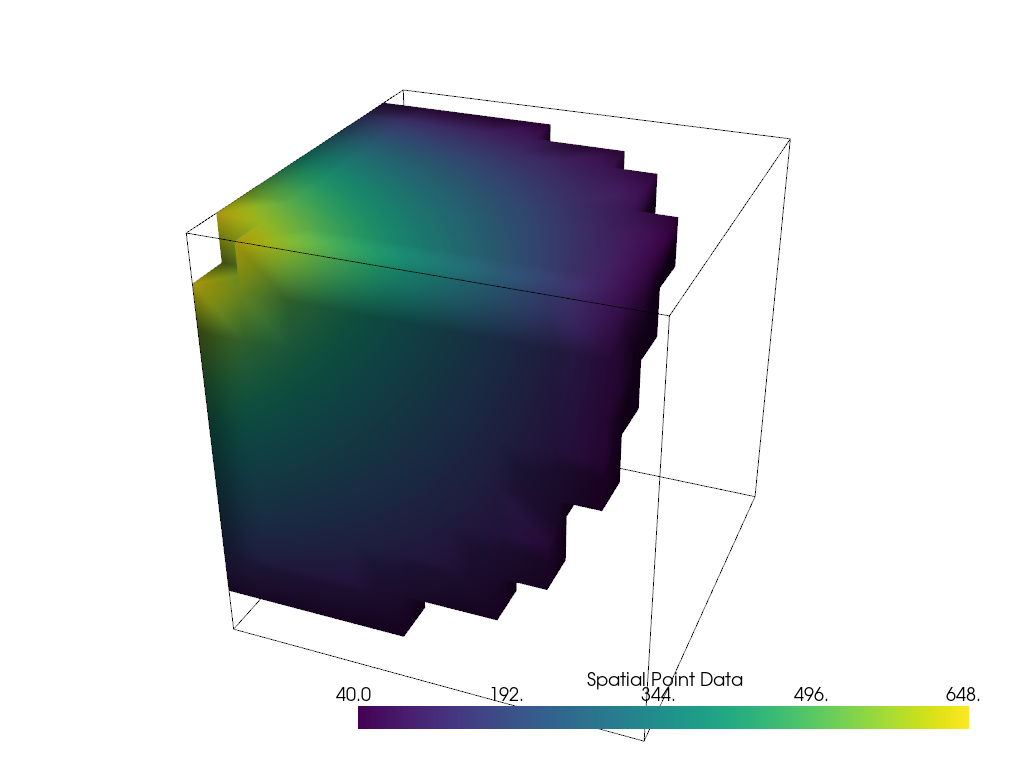
dataset.set_active_scalars("Spatial Point Data")
# Apply a threshold over a data range
threshed = dataset.threshold([100, 500])
outline = dataset.outline()
And now there is a thresholded version of the input dataset in the new
threshed object. To learn more about what keyword arguments are available to
alter how filters are executed, print the docstring for any filter attached to
PyVista objects with either help(dataset.threshold) or using shift+tab
in an IPython environment.
We can now plot this filtered dataset along side an outline of the original dataset:
pl = pv.Plotter()
pl.add_mesh(outline, color="k")
pl.add_mesh(threshed)
pl.camera_position = [-2, 5, 3]
pl.show()
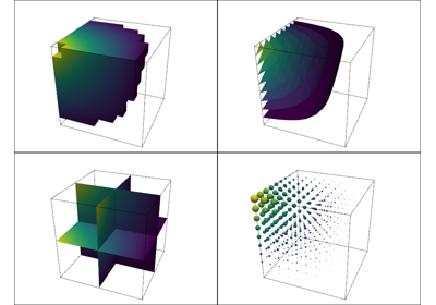
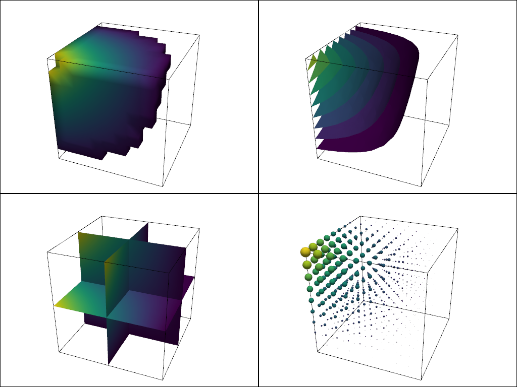
What about other filters? Let’s collect a few filter results and compare them:
import pyvista as pv
from pyvista import examples

dataset = examples.load_uniform()
outline = dataset.outline()
threshed = dataset.threshold([100, 500])
contours = dataset.contour()
slices = dataset.slice_orthogonal()
glyphs = dataset.glyph(factor=1e-3, geom=pv.Sphere(), orient=False)

pl = pv.Plotter(shape=(2, 2))
# Show the threshold
pl.add_mesh(outline, color="k")
pl.add_mesh(threshed, show_scalar_bar=False)
pl.camera_position = [-2, 5, 3]
# Show the contour
pl.subplot(0, 1)
pl.add_mesh(outline, color="k")
pl.add_mesh(contours, show_scalar_bar=False)
pl.camera_position = [-2, 5, 3]
# Show the slices
pl.subplot(1, 0)
pl.add_mesh(outline, color="k")
pl.add_mesh(slices, show_scalar_bar=False)
pl.camera_position = [-2, 5, 3]
# Show the glyphs
pl.subplot(1, 1)
pl.add_mesh(outline, color="k")
pl.add_mesh(glyphs, show_scalar_bar=False)
pl.camera_position = [-2, 5, 3]

pl.link_views()
pl.show()
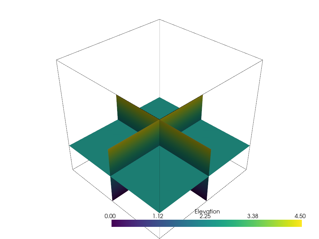
Filter Pipeline#
In VTK, filters are often used in a pipeline where each algorithm passes its output to the next filtering algorithm. In PyVista, we can mimic the filtering pipeline through a chain; attaching each filter to the last filter. In the following example, several filters are chained together:
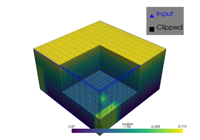
First, and empty
thresholdfilter to clean out anyNaNvalues.Use an
elevationfilter to generate scalar values corresponding to height.Use the
clipfilter to cut the dataset in half.Create three slices along each axial plane using the
slice_orthogonalfilter.
Apply a filtering chain
result = dataset.threshold().elevation().clip(normal="z").slice_orthogonal()
And to view this filtered data, simply call the plot method
(result.plot()) or create a rendering scene:
pl = pv.Plotter()
pl.add_mesh(outline, color="k")
pl.add_mesh(result, scalars="Elevation")
pl.view_isometric()
pl.show()