Contouring

Generate iso-lines or -surfaces for the scalars of a surface or volume.

3D meshes can have 2D iso-surfaces of a scalar field extracted and 2D surface meshes can have 1D iso-lines of a scalar field extracted.

import numpy as np
import pyvista as pv
from pyvista import examples

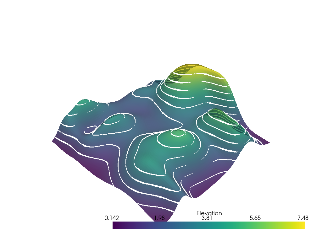
Iso-Lines

Let’s extract 1D iso-lines of a scalar field from a 2D surface mesh.

mesh = examples.load_random_hills()

help(mesh.contour)

Help on method contour in module pyvista.core.filters.data_set:

contour(isosurfaces=10, scalars=None, compute_normals=False, compute_gradients=False, compute_scalars=True, rng=None, preference='point', method='contour', progress_bar=False) method of pyvista.core.pointset.PolyData instance
    Contour an input self by an array.

    ``isosurfaces`` can be an integer specifying the number of
    isosurfaces in the data range or a sequence of values for
    explicitly setting the isosurfaces.

    Parameters
    ----------
    isosurfaces : int | sequence[float], optional
        Number of isosurfaces to compute across valid data range or a
        sequence of float values to explicitly use as the isosurfaces.

    scalars : str | array_like[float], optional
        Name or array of scalars to threshold on. If this is an array, the
        output of this filter will save them as ``"Contour Data"``.
        Defaults to currently active scalars.

    compute_normals : bool, default: False
        Compute normals for the dataset.

    compute_gradients : bool, default: False
        Compute gradients for the dataset.

    compute_scalars : bool, default: True
        Preserves the scalar values that are being contoured.

    rng : sequence[float], optional
        If an integer number of isosurfaces is specified, this is
        the range over which to generate contours. Default is the
        scalars array's full data range.

    preference : str, default: "point"
        When ``scalars`` is specified, this is the preferred array
        type to search for in the dataset.  Must be either
        ``'point'`` or ``'cell'``.

    method : str, default:  "contour"
        Specify to choose which vtk filter is used to create the contour.
        Must be one of ``'contour'``, ``'marching_cubes'`` and
        ``'flying_edges'``.

    progress_bar : bool, default: False
        Display a progress bar to indicate progress.

    Returns
    -------
    pyvista.PolyData
        Contoured surface.

    Examples
    --------
    Generate contours for the random hills dataset.

    >>> from pyvista import examples
    >>> hills = examples.load_random_hills()
    >>> contours = hills.contour()
    >>> contours.plot(line_width=5)

    Generate the surface of a mobius strip using flying edges.

    >>> import pyvista as pv
    >>> a = 0.4
    >>> b = 0.1
    >>> def f(x, y, z):
    ...     xx = x * x
    ...     yy = y * y
    ...     zz = z * z
    ...     xyz = x * y * z
    ...     xx_yy = xx + yy
    ...     a_xx = a * xx
    ...     b_yy = b * yy
    ...     return (
    ...         (xx_yy + 1) * (a_xx + b_yy)
    ...         + zz * (b * xx + a * yy)
    ...         - 2 * (a - b) * xyz
    ...         - a * b * xx_yy
    ...     ) ** 2 - 4 * (xx + yy) * (a_xx + b_yy - xyz * (a - b)) ** 2
    ...
    >>> n = 100
    >>> x_min, y_min, z_min = -1.35, -1.7, -0.65
    >>> grid = pv.ImageData(
    ...     dimensions=(n, n, n),
    ...     spacing=(
    ...         abs(x_min) / n * 2,
    ...         abs(y_min) / n * 2,
    ...         abs(z_min) / n * 2,
    ...     ),
    ...     origin=(x_min, y_min, z_min),
    ... )
    >>> x, y, z = grid.points.T
    >>> values = f(x, y, z)
    >>> out = grid.contour(
    ...     1,
    ...     scalars=values,
    ...     rng=[0, 0],
    ...     method='flying_edges',
    ... )
    >>> out.plot(color='lightblue', smooth_shading=True)

    See :ref:`common_filter_example` or
    :ref:`marching_cubes_example` for more examples using this
    filter.

contours = mesh.contour()

p = pv.Plotter()
p.add_mesh(mesh, opacity=0.85)
p.add_mesh(contours, color="white", line_width=5)
p.show()

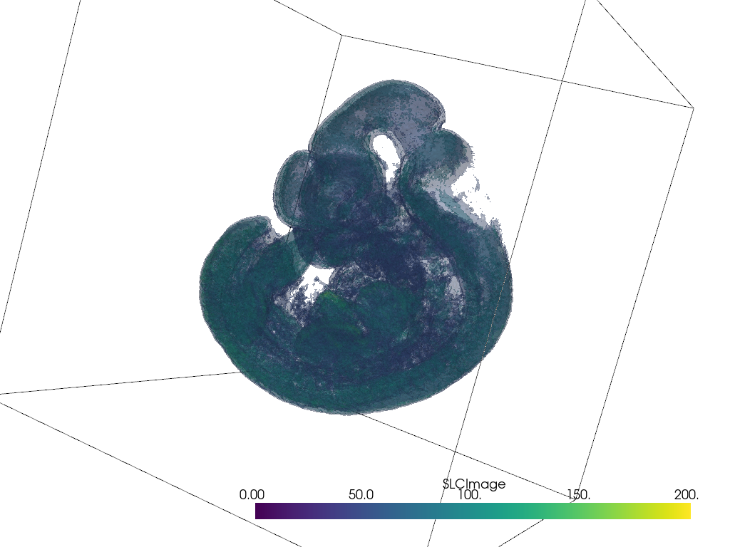
Iso-Surfaces

Let’s extract 2D iso-surfaces of a scalar field from a 3D mesh.

mesh = examples.download_embryo()
mesh

Header	Data Arrays
ImageData Information N Cells 16581375 N Points 16777216 X Bounds 0.000e+00, 2.550e+02 Y Bounds 0.000e+00, 2.550e+02 Z Bounds 0.000e+00, 2.550e+02 Dimensions 256, 256, 256 Spacing 1.000e+00, 1.000e+00, 1.000e+00 N Arrays 1	Name Field Type N Comp Min Max SLCImage Points uint8 1 0.000e+00 1.970e+02

For this example dataset, let’s create 5 contour levels between the values of 50 and 200

contours = mesh.contour(np.linspace(50, 200, 5))

p = pv.Plotter()
p.add_mesh(mesh.outline(), color="k")
p.add_mesh(contours, opacity=0.25, clim=[0, 200])
p.camera_position = [
    (-130.99381142132086, 644.4868354828589, 163.80447435848686),
    (125.21748748157661, 123.94368717158413, 108.83283586619626),
    (0.2780372840777734, 0.03547871361794171, 0.9599148553609699),
]
p.show()