Plotting Options and Animations#

Demonstrate many features of the PyVista plotting API to create compelling 3D visualizations and touch on animations (10 min for talk, 10 min for exercise)

Tip

This section of the tutorial was adopted from the Plotting section of PyVista’s Example Gallery.

PyVista enables many possibilities for altering how you display 3D data, a few of our most common features include:

Color mapping scalar values with Matplotlib colormaps
Showing the edges and nodes of different mesh types
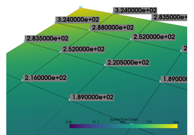
Label points in 3D space along side your meshes
Creating side-by-side comparisons
Making a dataset transparent or using a scalar value to map opacity
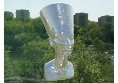
Adding textures/images draped over a mesh (texture mapping)
Use sophisticated lighting techniques like smooth shading or Eye Dome Lighting
Creating animations as GIFs or movie files

This section will overview PyVista’s pyvista.Plotter API and how to perform these tasks. The goal of this lesson is not to be a comprehensive overview of PyVista’s plotting API, but rather to demonstrate how it works and how you can learn to use it!

The Basics#

PyVista’s plotting API is data-centric, where the 3D data are individually added to the scene with different display parameters in a Matplotlib-like fashion.

Add Mesh to Plotter Object#

When plotting, users must first create a pyvista.Plotter instance (much like a Matplotlib figure). Then data are added to the plotter instance through the pyvista.Plotter.add_mesh() method. This workflow typically looks like:

import pyvista as pv
from pyvista import examples

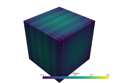
mesh = pv.Wavelet()

p = pv.Plotter()
p.add_mesh(mesh)
p.show()

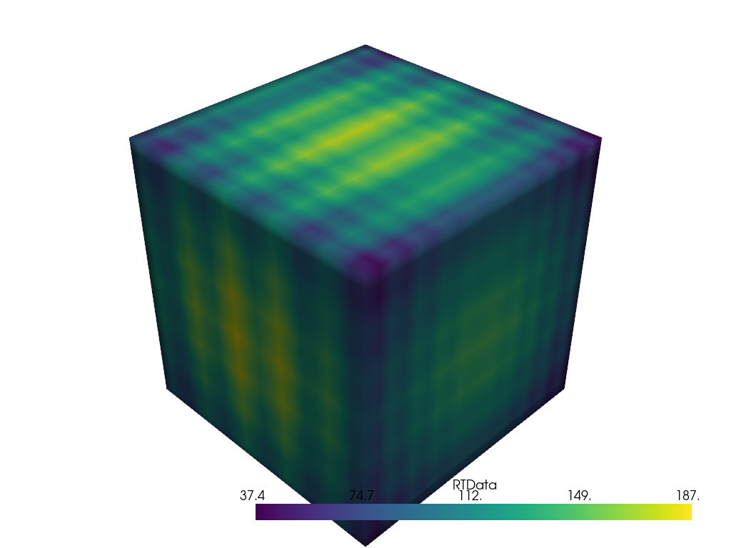
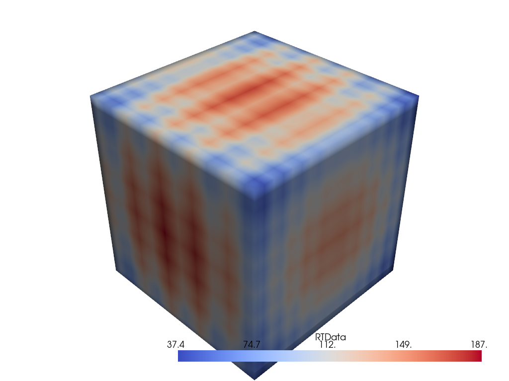
You can customize how that mesh is displayed through the parameters of the pyvista.Plotter.add_mesh() method. For example, we can change the colormap via the cmap argument:

p = pv.Plotter()
p.add_mesh(mesh, cmap='coolwarm')
p.show()

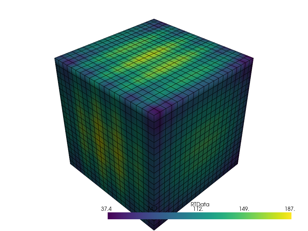
Or show the edges of the mesh with show_edges:

p = pv.Plotter()
p.add_mesh(mesh, show_edges=True)
p.show()

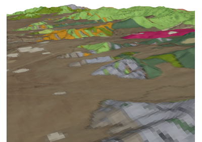
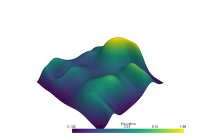
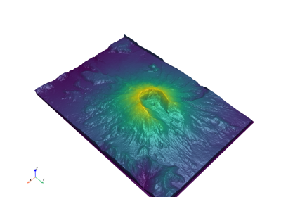
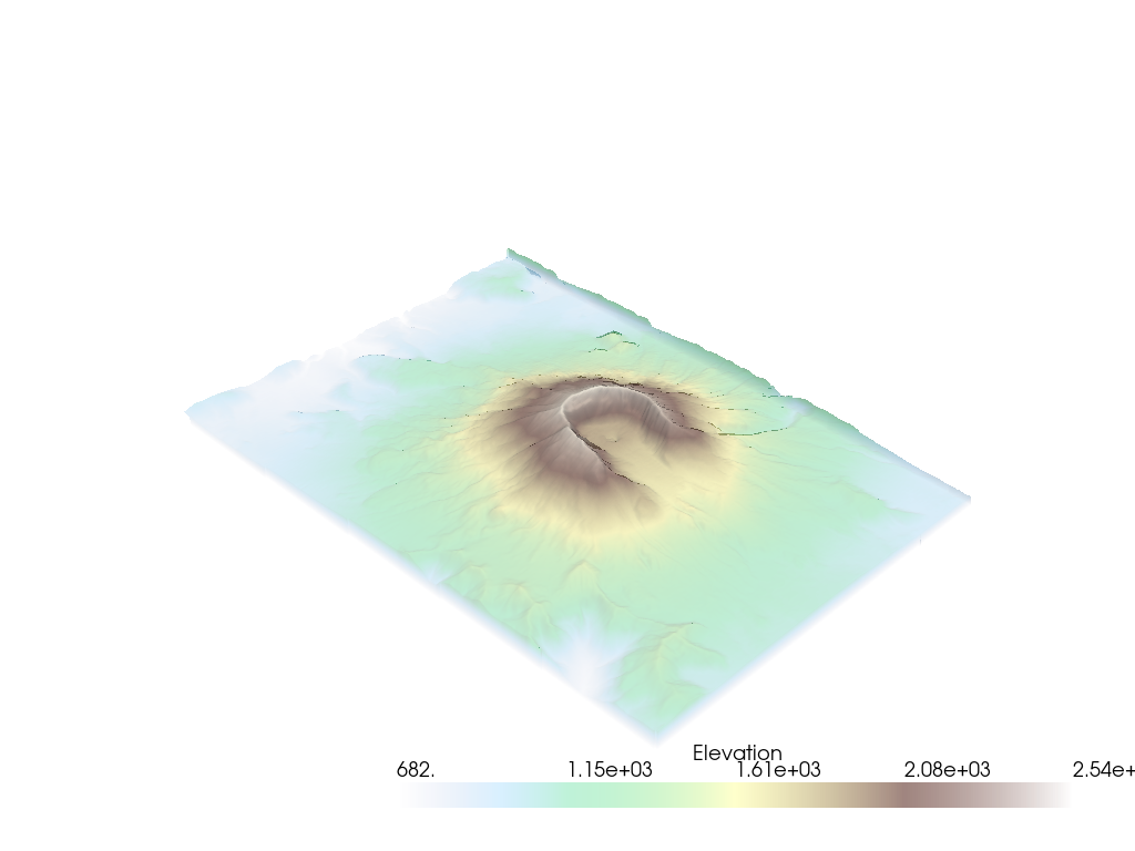
Or adjust the opacity to be a scalar value or linear transfer function via the opacity argument:

import pyvista as pv
from pyvista import examples

mesh = examples.download_st_helens().warp_by_scalar()

p = pv.Plotter()
p.add_mesh(mesh, cmap='terrain', opacity="linear")
p.show()

Take a look at all of the options for add_mesh.

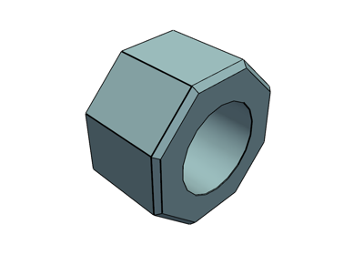
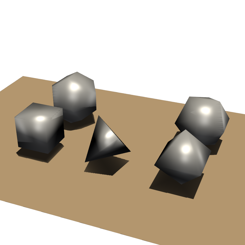
The add_mesh method can be called over and over to add different data to the same Plotter scene. For example, we can create many different mesh objects and plot them together:

import pyvista as pv
from pyvista import examples

kinds = [
    'tetrahedron',
    'cube',
    'octahedron',
    'dodecahedron',
    'icosahedron',
]
centers = [
    (0, 1, 0),
    (0, 0, 0),
    (0, 2, 0),
    (-1, 0, 0),
    (-1, 2, 0),
]

solids = [pv.PlatonicSolid(kind, radius=0.4, center=center) for kind, center in zip(kinds, centers)]

p = pv.Plotter(window_size=[1000, 1000])
for solid in solids:
    p.add_mesh(
        solid, color='silver', specular=1.0, specular_power=10
    )
p.view_vector((5.0, 2, 3))
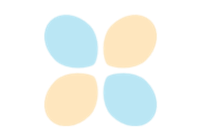
p.add_floor('-z', lighting=True, color='tan', pad=1.0)
p.enable_shadows()
p.show()

Subplotting#

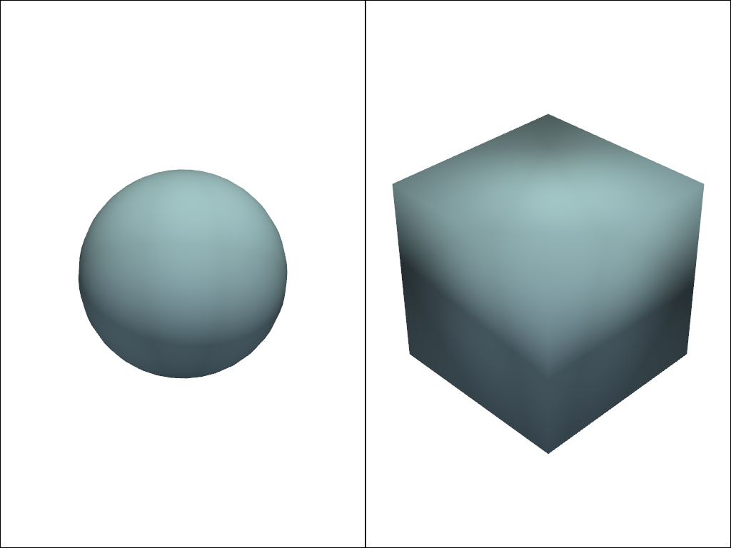
Creating side-by-side comparisons of datasets is easy with PyVista’s subplotting API. Get started by specifying the shape of the pyvista.Plotter object then registering the active subplot by the pyvista.Plotter.subplot() method much like how you subplot with Matplotlib’s API.

import pyvista as pv

p = pv.Plotter(shape=(1, 2))

p.subplot(0, 0)
p.add_mesh(pv.Sphere())

p.subplot(0, 1)
p.add_mesh(pv.Cube())

p.show()

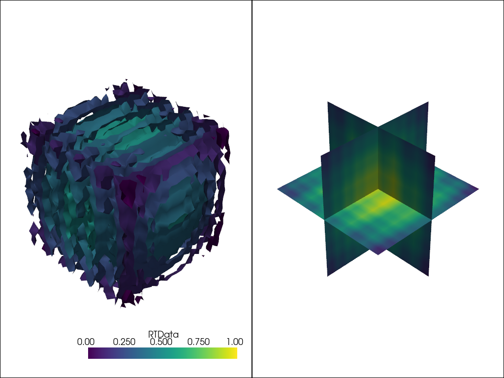
Below is an example of side-by-side comparisons of the contours and slices of a single dataset.

Tip

You can link the cameras of both views with the pyvista.Plotter.link_views() method

import pyvista as pv

mesh = pv.Wavelet()
cntr = mesh.contour()
slices = mesh.slice_orthogonal()

p = pv.Plotter(shape=(1, 2))

p.add_mesh(cntr)

p.subplot(0, 1)
p.add_mesh(slices)

p.link_views()
p.view_isometric()
p.show()

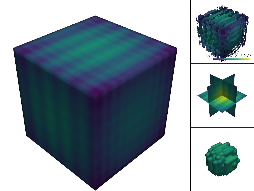
Other custom layouts are supported by the shape argument as string descriptors:

shape="3|1" means 3 plots on the left and 1 on the right,
shape="4/2" means 4 plots on top and 2 at the bottom.

Here is an example of three plots on the right and one on the left:

import pyvista as pv

mesh = pv.Wavelet()
cntr = mesh.contour()
slices = mesh.slice_orthogonal()
thresh = mesh.threshold(200)

p = pv.Plotter(shape="1|3")

p.subplot(1)
p.add_mesh(cntr)

p.subplot(2)
p.add_mesh(slices)

p.subplot(3)
p.add_mesh(thresh)

p.subplot(0)
p.add_mesh(mesh)

p.link_views()
p.view_isometric()
p.show()

Note

There is a comprehensive overview of subplotting in the Multi-Window Plotting Example This example details how to create more complex layouts.

Controlling the Scene#

Tip

For a full list of methods on the pyvista.Plotter, please see the API documentation

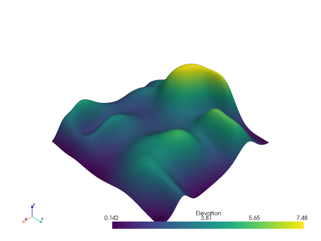
Axes and Bounds#

Axes can be added to the scene with pyvista.Plotter.show_axes()

import pyvista as pv
from pyvista import examples

mesh = examples.load_random_hills()

p = pv.Plotter()
p.add_mesh(mesh)
p.show_axes()
p.show()

And bounds similarly with pyvista.Plotter.show_bounds()

Tip

See Plotting Bounds for more details.

import pyvista as pv
from pyvista import examples

mesh = examples.load_random_hills()

p = pv.Plotter()
p.add_mesh(mesh)
p.show_axes()
p.show_bounds()
p.show()