Lesson Overview

import pyvista as pv
from pyvista import examples

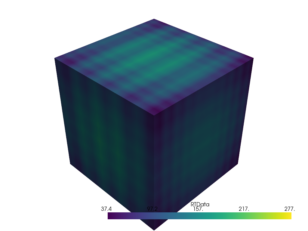
mesh = pv.Wavelet()

add_mesh

When plotting, users must first create a pyvista.Plotter instance (much like a Matplotlib figure). Then data are added to the plotter instance through the pyvista.Plotter.add_mesh() method. This workflow typically looks like:

p = pv.Plotter()
p.add_mesh(mesh)
p.show()

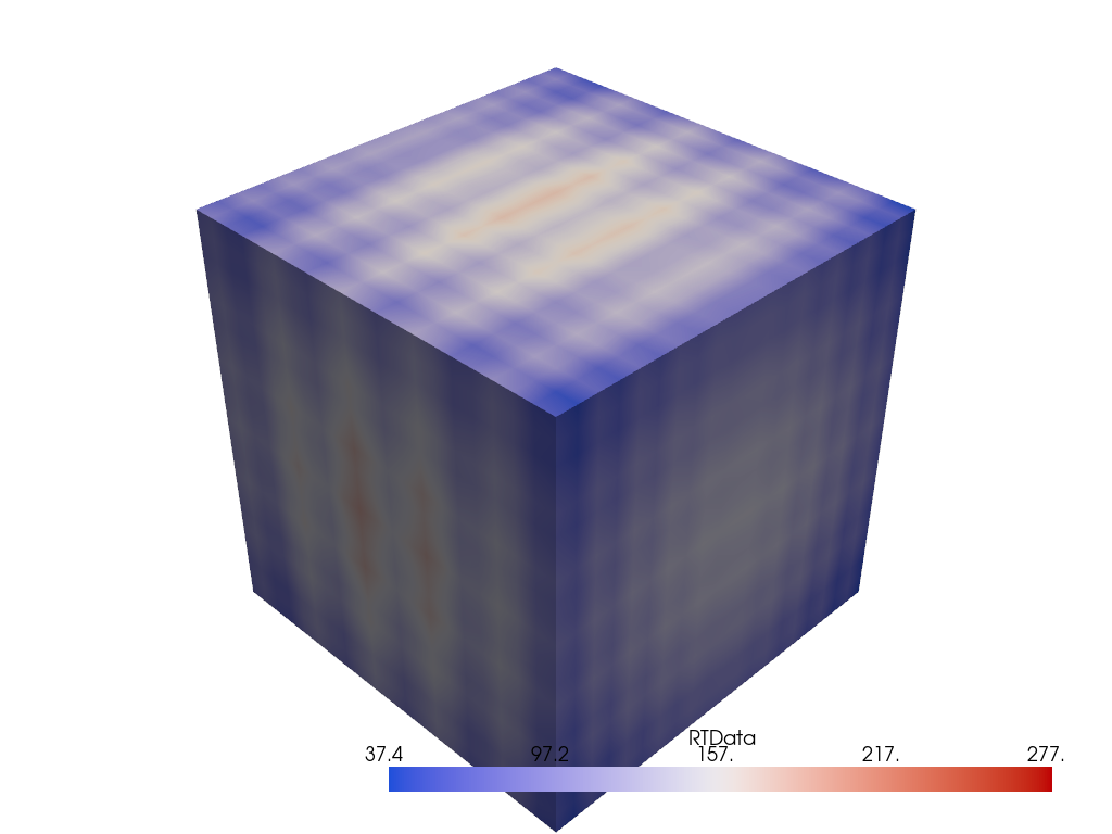
You can customize how that mesh is displayed through the parameters of the pyvista.Plotter.add_mesh() method. For example, we can change the colormap via the cmap argument:

p = pv.Plotter()
p.add_mesh(mesh, cmap='coolwarm')
p.show()

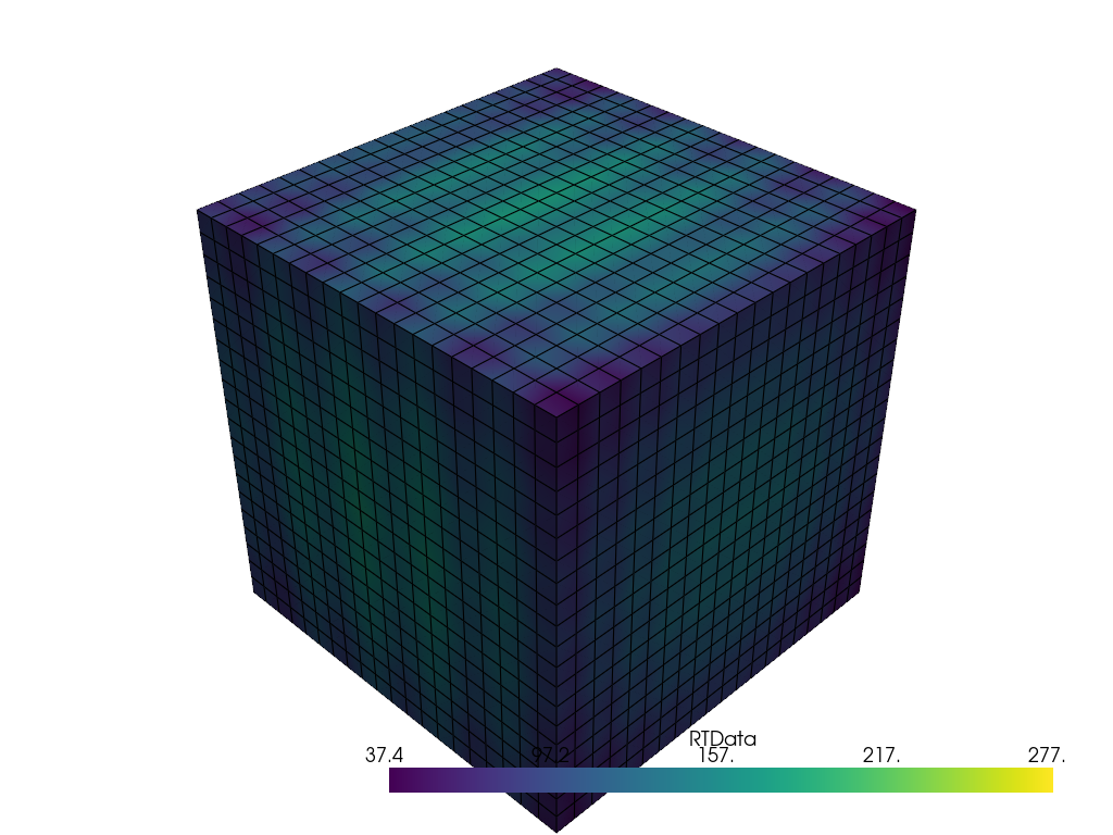
Or show the edges of the mesh with show_edges:

p = pv.Plotter()
p.add_mesh(mesh, show_edges=True)
p.show()

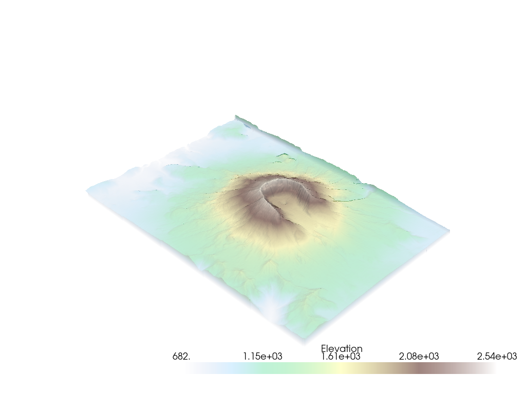
Or adjust the opacity to be a scalar value or linear transfer function via the opacity argument:

mesh = examples.download_st_helens().warp_by_scalar()

p = pv.Plotter()
p.add_mesh(mesh, cmap='terrain', opacity="linear")
p.show()

Take a look at all of the options for add_mesh.

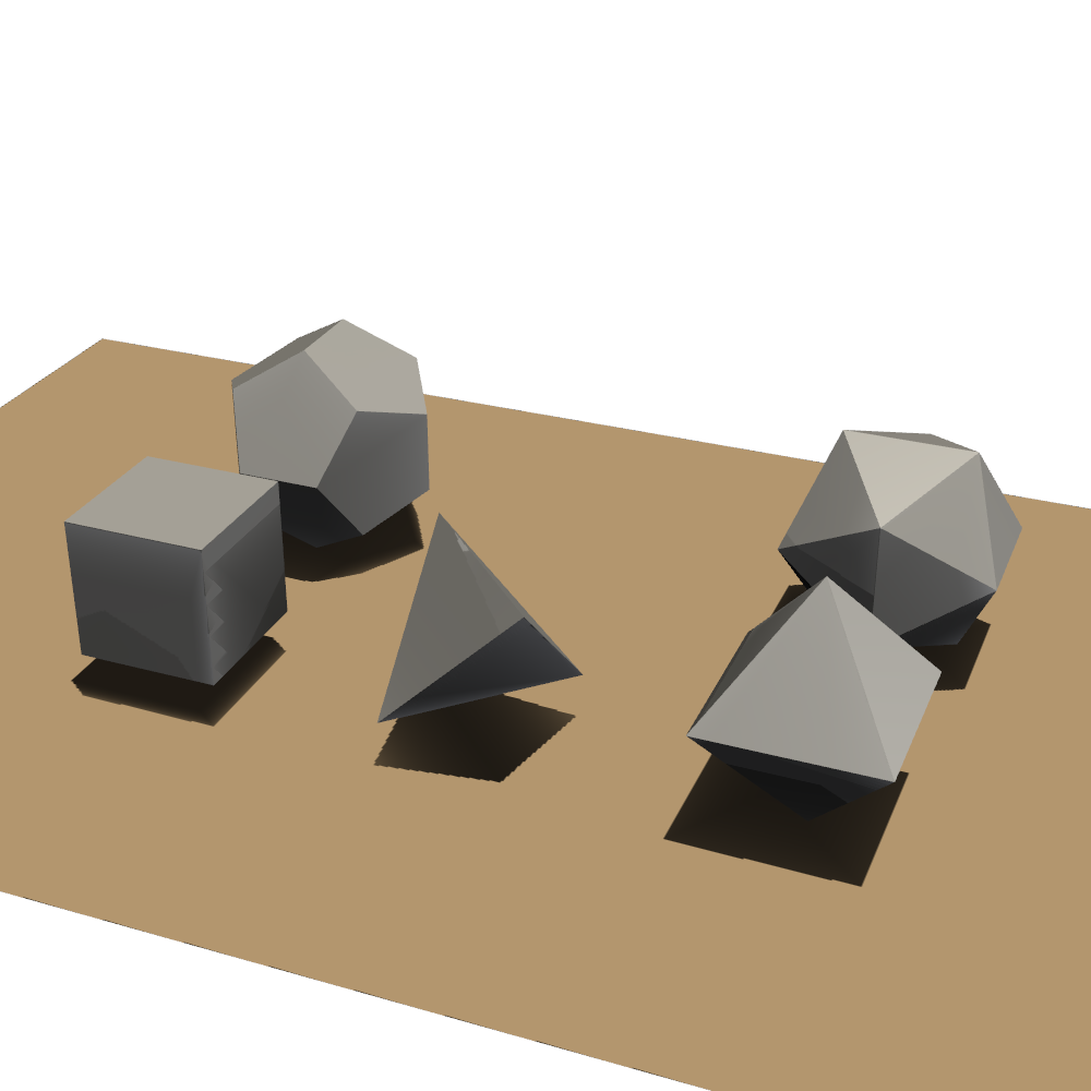
The add_mesh method can be called over and over to add different data to the same Plotter scene. For example, we can create many different mesh objects and plot them together:

kinds = [
    'tetrahedron',
    'cube',
    'octahedron',
    'dodecahedron',
    'icosahedron',
]
centers = [
    (0, 1, 0),
    (0, 0, 0),
    (0, 2, 0),
    (-1, 0, 0),
    (-1, 2, 0),
]

solids = [pv.PlatonicSolid(kind, radius=0.4, center=center) for kind, center in zip(kinds, centers)]

p = pv.Plotter(window_size=[1000, 1000])
for ind, solid in enumerate(solids):
    p.add_mesh(solid, color='silver', specular=1.0, specular_power=10)
p.view_vector((5.0, 2, 3))
p.add_floor('-z', lighting=True, color='tan', pad=1.0)
p.enable_shadows()
p.show()

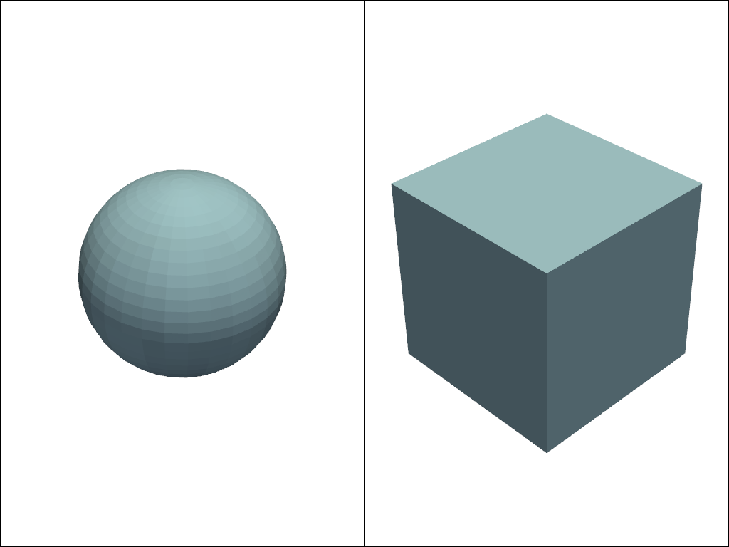
Subplotting

Creating side-by-side comparisons of datasets is easy with PyVista’s subplotting API. Get started by specifying the shape of the pyvista.Plotter object then registering the active subplot by the pyvista.Plotter.subplot() method much like how you subplot with Matplotlib’s API.

p = pv.Plotter(shape=(1, 2))

p.subplot(0, 0)
p.add_mesh(pv.Sphere())

p.subplot(0, 1)
p.add_mesh(pv.Cube())

p.show()

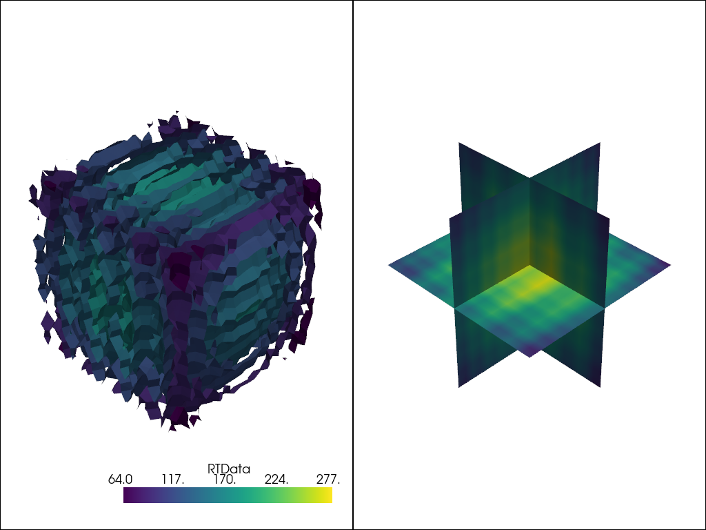
Below is an example of side-by-side comparisons of the contours and slices of a single dataset.

Tip

You can link the cameras of both views with the pyvista.Plotter.link_views() method

mesh = pv.Wavelet()
cntr = mesh.contour()
slices = mesh.slice_orthogonal()

p = pv.Plotter(shape=(1, 2))

p.add_mesh(cntr)

p.subplot(0, 1)
p.add_mesh(slices)

p.link_views()
p.view_isometric()
p.show()

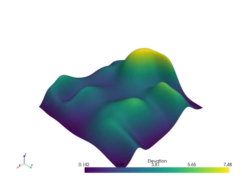
Axes and Bounds

Axes can be added to the scene with pyvista.Plotter.show_axes()

mesh = examples.load_random_hills()

p = pv.Plotter()
p.add_mesh(mesh)
p.show_axes()
p.show()

And bounds similarly with pyvista.Plotter.show_bounds()

Tip

See Plotting Bounds for more details.

p = pv.Plotter()
p.add_mesh(mesh)
p.show_axes()
p.show_bounds()
p.show()