Basic usage#
This section demonstrates how to use PyVista for reading and plotting 3D data using the pyvista.examples module and external files.
Tip
This section of the tutorial was adopted from the Basic API Usage chapter of the PyVista documentation.
Using Existing Data#
There are two main ways of getting data into PyVista: creating it yourself from scratch or loading the dataset from any one of the compatible file formats. Since we’re just starting out, let’s load a file.
If you have a dataset handy, like a surface model, point cloud, or VTK file, you can use that. If you don’t have something immediately available, PyVista has a variety of files you can download in its pyvista.examples.downloads module.
Here’s a very basic dataset you can download.
from pyvista import examples
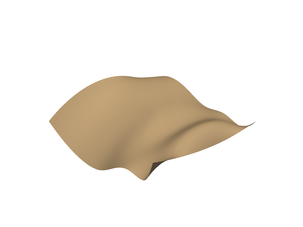
dataset = examples.download_saddle_surface()
dataset
Note how this is a pyvista.PolyData, which is effectively a surface
dataset containing points, lines, and/or faces. We can immediately plot this with:
dataset.plot(color='tan')
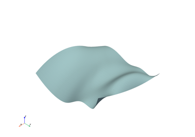
This is a fairly basic plot. You can change how its plotted by adding
parameters as show_edges=True or changing the color by setting color to
a different value. All of this is described in PyVista’s API documentation in
pyvista.plot(), but for now let’s take a look at another dataset. This
one is a volumetric dataset.
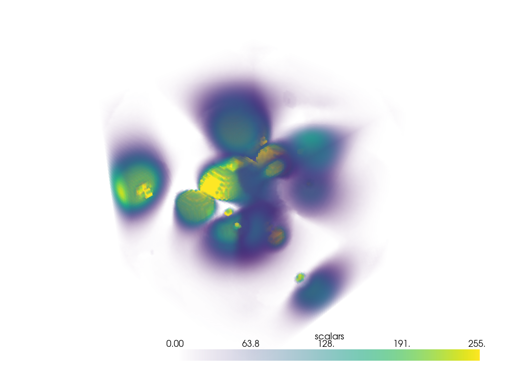
dataset = examples.download_frog()
dataset
This is a pyvista.ImageData, which is a dataset containing a uniform
set of points with consistent spacing. When we plot this dataset, we have the
option of enabling volumetric plotting, which plots individual cells based on
the content of the data associated with those cells.
dataset.plot(volume=True)
Note
One thing you might have noticed by now is that the plots here in the online
tutorial may look slightly different than your plots depending on how you’re plotting them
on your computer. This depends on your jupyter_backend, or if
you’re even using a jupyter notebook. As you’re playing around with these
examples, feel free to change settings like disabling (or enabling)
notebook, or using a different plotting backend for displaying within
your notebook (if applicable).
Read from a file#
You can read datasets directly from a file if you have access to it locally on your computer. This can be one of the many file formats that VTK supports, and many more that it doesn’t as PyVista can rely on libraries like meshio.
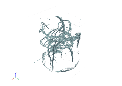
In the following example, we load VTK’s iron protein dataset ironProt.vtk from a
file using pyvista.read().
import pyvista as pv
dataset = pv.read('ironProt.vtk')
dataset
This is again a pyvista.ImageData and we can plot it volumetrically
with:
dataset.plot(volume=True)
Lesson Material#
This is the notebook rendering of this page where you can interactively follow along with this lesson.
Exercises#

Solutions#
These are the solutions to the above examples.