Lesson Overview

This exercise provides an overview of the example in the initial lesson for you to try out!

import numpy as np
import pyvista as pv
from pyvista import examples

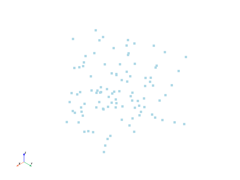
What is a Point?

Let’s start with a point cloud – this is a mesh type that only has vertices. You can create one by defining a 2D array of Cartesian coordinates like so:

points = np.random.rand(100, 3)
points[:5, :]  # output first 5 rows

array([[0.29317083, 0.78732679, 0.15095965],
       [0.50576457, 0.16839412, 0.0695445 ],
       [0.00471359, 0.92851619, 0.11911979],
       [0.37926714, 0.74415264, 0.91484657],
       [0.56020373, 0.88690684, 0.04575484]])

Pass numpy array of points (n by 3) to PolyData

mesh = pv.PolyData(points)
mesh

PolyData	Information
N Cells	100
N Points	100
N Strips	0
X Bounds	4.714e-03, 9.977e-01
Y Bounds	2.567e-03, 9.955e-01
Z Bounds	1.893e-02, 9.980e-01
N Arrays	0

mesh.plot(point_size=10, style="points")

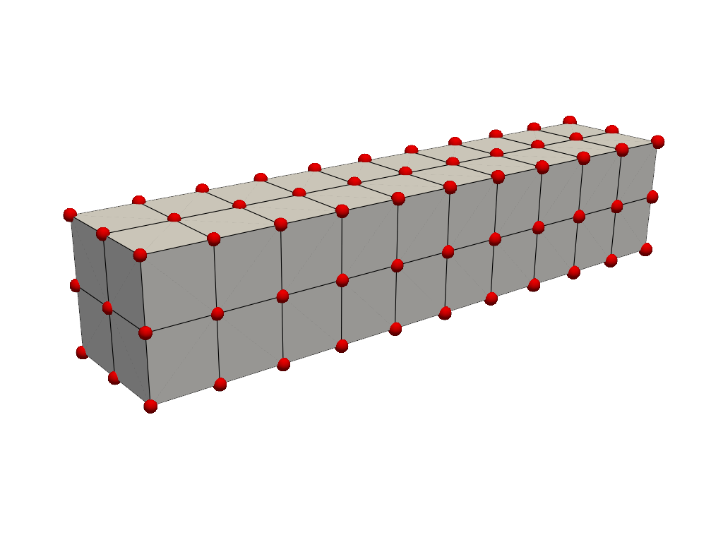
But it’s important to note that most meshes have some sort of connectivity between points such as this gridded mesh:

mesh = examples.load_hexbeam()
cpos = [(6.20, 3.00, 7.50), (0.16, 0.13, 2.65), (-0.28, 0.94, -0.21)]

pl = pv.Plotter()
pl.add_mesh(mesh, show_edges=True, color="white")
pl.add_points(mesh.points, color="red", point_size=20, render_points_as_spheres=True)
pl.camera_position = cpos
pl.show()

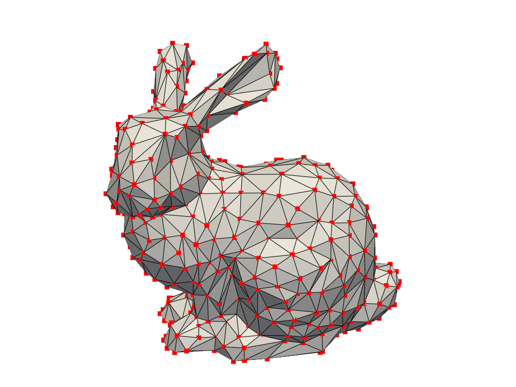
mesh = examples.download_bunny_coarse()

pl = pv.Plotter()
pl.add_mesh(mesh, show_edges=True, color="white")
pl.add_points(mesh.points, color="red", point_size=10)
pl.camera_position = [(0.02, 0.30, 0.73), (0.02, 0.03, -0.022), (-0.03, 0.94, -0.34)]
pl.show()

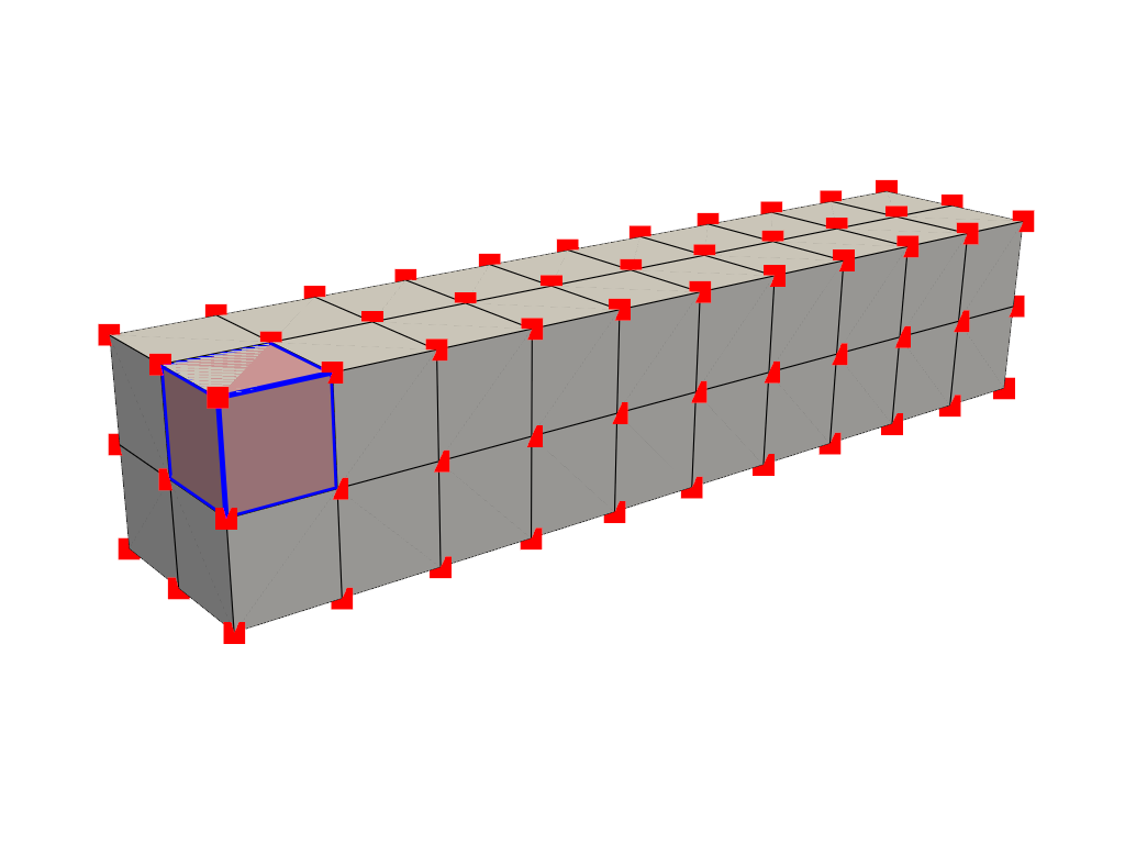
What is a Cell?

A cell is the geometry between points that defines the connectivity or topology of a mesh. In the examples above, cells are defined by the lines (edges colored in black) connecting points (colored in red). For example, a cell in the beam example is a voxel defined by the region between eight points in that mesh:

mesh = examples.load_hexbeam()

pl = pv.Plotter()
pl.add_mesh(mesh, show_edges=True, color="white")
pl.add_points(mesh.points, color="red", point_size=20)

single_cell = mesh.extract_cells(mesh.n_cells - 1)
pl.add_mesh(single_cell, color="pink", edge_color="blue", line_width=5, show_edges=True)

pl.camera_position = [(6.20, 3.00, 7.50), (0.16, 0.13, 2.65), (-0.28, 0.94, -0.21)]
pl.show()

Cells aren’t limited to voxels, they could be a triangle between three points, a line between two points, or even a single point could be its own cell (but that’s a special case).

What are attributes?

Attributes are data values that live on either the points or cells of a mesh. In PyVista, we work with both point data and cell data and allow easy access to data dictionaries to hold arrays for attributes that live either on all points or on all cells of a mesh. These attributes can be accessed in a dictionary-like attribute attached to any PyVista mesh accessible as one of the following:

Point Data

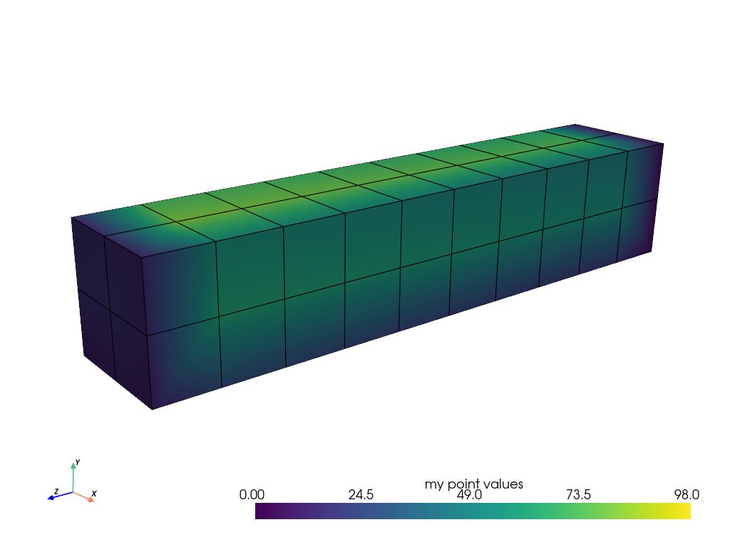
Point data refers to arrays of values (scalars, vectors, etc.) that live on each point of the mesh. Each element in an attribute array corresponds to a point in the mesh. Let’s create some point data for the beam mesh. When plotting, the values between points are interpolated across the cells.

mesh.point_data["my point values"] = np.arange(mesh.n_points)
mesh.plot(scalars="my point values", cpos=cpos, show_edges=True)

Cell Data

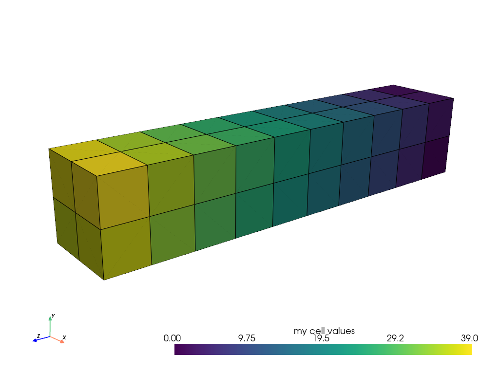
Cell data refers to arrays of values (scalars, vectors, etc.) that live throughout each cell of the mesh. That is the entire cell (2D face or 3D volume) is assigned the value of that attribute.

mesh.cell_data["my cell values"] = np.arange(mesh.n_cells)
mesh.plot(scalars="my cell values", cpos=cpos, show_edges=True)

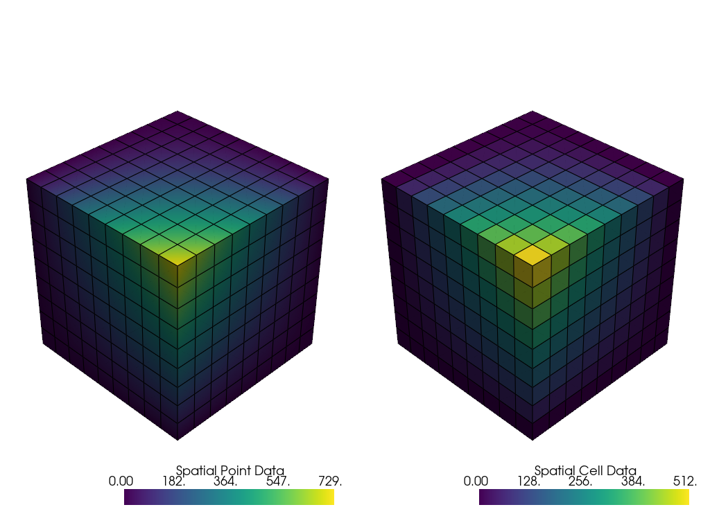
Here’s a comparison of point data versus cell data and how point data is interpolated across cells when mapping colors. This is unlike cell data which has a single value across the cell’s domain:

import pyvista as pv
from pyvista import examples

uni = examples.load_uniform()

pl = pv.Plotter(shape=(1, 2), border=False)
pl.add_mesh(uni, scalars="Spatial Point Data", show_edges=True)
pl.subplot(0, 1)
pl.add_mesh(uni, scalars="Spatial Cell Data", show_edges=True)
pl.link_views()
pl.show()

Field Data

Field data is not directly associated with either the points or cells but still should be attached to the mesh. This may be a string array storing notes.

mesh = pv.Cube()
mesh.field_data['metadata'] = ['Foo', 'bar']
mesh.field_data

pyvista DataSetAttributes
Association     : NONE
Contains arrays :
    metadata                <U3        (2,)

Assigning Scalars to a Mesh

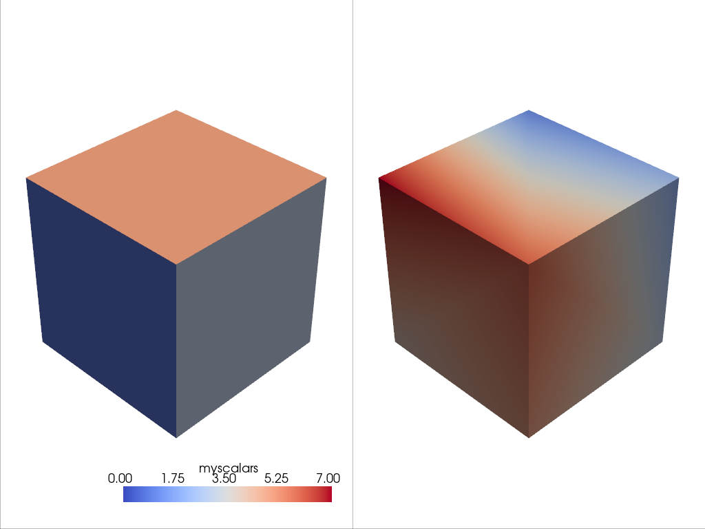
Here’s how we assign values to cell attributes and plot it. Here, we generate cube containing 6 faces and assign each face an integer from range(6) and then have it plotted.

Note how this varies from assigning scalars to each point

cube = pv.Cube()
cube.cell_data["myscalars"] = range(6)

other_cube = cube.copy()
other_cube.point_data["myscalars"] = range(8)

pl = pv.Plotter(shape=(1, 2), border_width=1)
pl.add_mesh(cube, cmap="coolwarm")
pl.subplot(0, 1)
pl.add_mesh(other_cube, cmap="coolwarm")
pl.show()